Cells

import numpy as np
import matplotlib.pyplot as plt
import pandas as pd
from PIL import Image
from PIL import ImageEnhance

from imagemks.rw import rwformat
from imagemks.workflows import segment_fluor_cells, measure_fluor_cells, visualize_fluor_cells
from imagemks.workflows import default_parameters

import warnings
warnings.filterwarnings("ignore")

Setting up the parameters and loaders

path_to_data = '/home/sven/Projects/data/cells/'
zoomLev = 2
p = default_parameters('muscle')

nucs_loader = rwformat(path_to_data, prefix='b', ftype='.jpg')
cyto_loader = rwformat(path_to_data, prefix='g', ftype='.jpg')

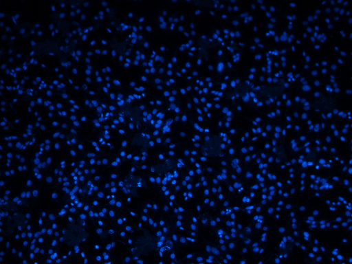
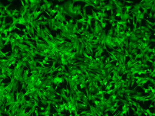
Loading the original images

n = 12

N = nucs_loader[n]
C = cyto_loader[n]

small_size = [i//5 for i in N.size]

N.resize(small_size)

C.resize(small_size)

Running the Segmentation

N = np.sum(np.array(N), axis=2)
C = np.sum(np.array(C), axis=2)
S_N, S_C = segment_fluor_cells(N, C, p['smooth_size'], p['intensity_curve'], p['short_th_radius'],
                        p['long_th_radius'], p['min_frequency_to_remove'], p['max_frequency_to_remove'],
                        p['max_size_of_small_objects_to_remove'], p['peak_min_distance'],
                        p['size_after_watershed_to_remove'], p['cyto_local_avg_size'], zoomLev)

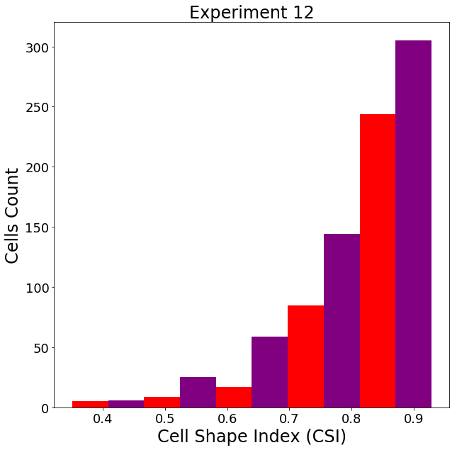
Extracting Measurements

df = measure_fluor_cells(S_N, S_C, pix_size=0.48) #pixel size in micrometers along edge of pixel

csi = 4*np.pi * (df['Nuc_Area_um2'].values / df['Nuc_Perimeter_um'].values**2)

hist, bins = np.histogram(csi, bins=10)

colors = ['red','purple']*5

fig, ax = plt.subplots(1,1, figsize=(10,10))
ax.bar(bins[:-1], hist, width=(bins[1]-bins[0]), color=colors)#, c='red')#, align='edge')
ax.set_title('Experiment %d'%n, fontsize=24)
ax.set_xlabel('Cell Shape Index (CSI)', fontsize=24)
ax.set_ylabel('Cells Count', fontsize=24)
for tick in ax.xaxis.get_major_ticks():
    tick.label.set_fontsize(18)
for tick in ax.yaxis.get_major_ticks():
    tick.label.set_fontsize(18)
plt.show(fig)

V_N, E_N = visualize_fluor_cells(S_N, N)

V_N = Image.fromarray(V_N).resize(small_size)
E_N = Image.fromarray(E_N).resize(small_size)

V_C, E_C = visualize_fluor_cells(S_C, C)

V_C = Image.fromarray(V_C).resize(small_size)
E_C = Image.fromarray(E_C).resize(small_size)

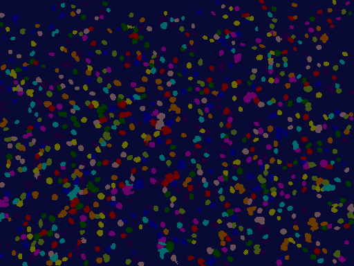
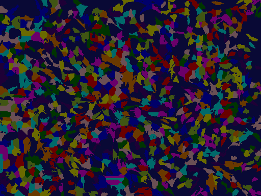
Showing the colored segmentations

The colors of both images correspond to each other. For each nucleus in the segmented nucleus image, the cytoskeleton was assigned an identical label and color.

V = ImageEnhance.Brightness(V_N)
V.enhance(1.4)

V = ImageEnhance.Brightness(V_C)
V.enhance(1.4)

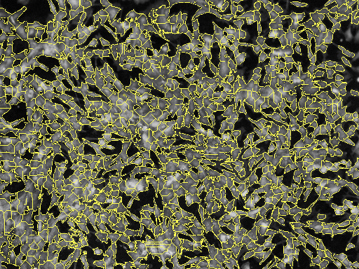
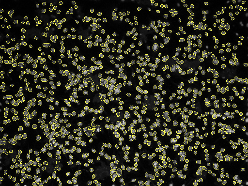
Showing borders

Borders are important to detect because a good border gives a better measurement. Measurements such as cell shape index (CSI) are important in identifying the type of cell. A CSI of greater than 0.8 shows that we have muscle cells, which is true for experiment 9.

E_N

E_C